In this paper, we consider the optimal source control problem of a system of 2-dimensional semi-linear steady convection-diffusion equations. The problem is modelized from temperature and consistency distribution in the gasification processes, so it is described by 2 non-linear elliptic partial differential equations with Dirichlet boundary condition. The problem is a optimal source control problem that controls the source term necessary to approximate the temperature to a proper target function. First, we derived the optimal condition. Based on setting the approximation problem of a given control problem in a first order polynomial finite element function space and deriving the optimality condition of the approximation problem, we evaluated a priori error between the optimal control, the optimal state, the conjugate state and its finite element approximation functions by using optimal condition of original and approximate problem. And we also evaluated the upper estimate of a posteriori error by finite element method (FEM). We proved the convergence to 0 of a posteriori error indicator (term of the right side of inequality) when division diameter converges to 0. For this, we acquired the lower bound estimation of a posteriori error and proved that a priori error and total variance error converges to 0 when division diameter converges to 0, so that we proved the convergence problem of a posteriori error indicator.
| Published in | International Journal of Industrial and Manufacturing Systems Engineering (Volume 10, Issue 2) |
| DOI | 10.11648/j.ijimse.20251002.11 |
| Page(s) | 20-35 |
| Creative Commons |
This is an Open Access article, distributed under the terms of the Creative Commons Attribution 4.0 International License (http://creativecommons.org/licenses/by/4.0/), which permits unrestricted use, distribution and reproduction in any medium or format, provided the original work is properly cited. |
| Copyright |
Copyright © The Author(s), 2025. Published by Science Publishing Group |
System of Semi-Linear Convection-Diffusion Equations, Source Control, A Posteriori Error Estimates

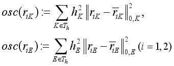
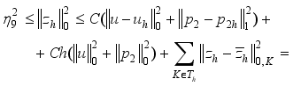
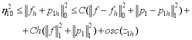
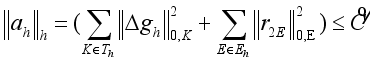
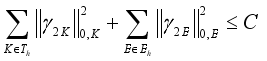
 (where K is patch of element in
  , E is edge of element in
  , s = 0, 1, 2).
 is bounded convex polygonal domain in
  and
and  is boundary of
  . The state model is as follows.
 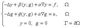 (1)
(1)  (2)
(2) 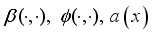 satisfy the following conditions.
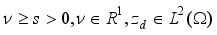 - is known.
 .
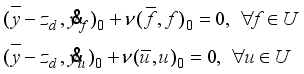
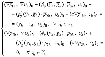
.  is the solution of problem 1. Then there exists a function
  so that it satisfies the following system.
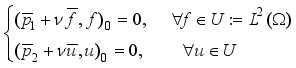
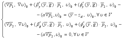 (3)
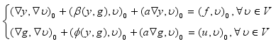
(3)  satisfy the following equations, respectively.
  (4)
(4)  (5)
(5)  of
of  , the solution of (2). Then , satisfy the following equations.
  (6)
(6)  (7)
(7)  (8)
(8)  (9)
(9)  (10)
(10)  (11)
(11)  (12)
(12)  (13)
(13)  (14)
(14)  (15)
(15)  (16)
(16) 
 from the fact that embedding is continuous. Therefore, we can obtain the result of this theorem.
  by , length of edge by ,
  . Let be the family of triangulation, be the set of edges of .

 isthelinearpolygonalspaceonelementK,
  .
.  (17)
(17) 
 is the unique solution of (17).
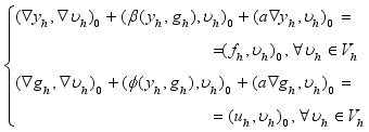
  is the solution of problem 2, there exists a
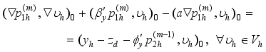
  so that it satisfies the following system of equations.
 (18)
(18)  is the unique solution of (17).
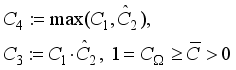
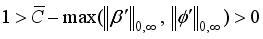
 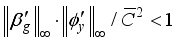 holds true. Then the equation (18) has a unique solution, where
  is the positive constant such that
 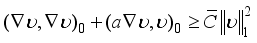 .
. 
 (19)
(19)  in every equations above.
  , from the above iteration scheme, we have
 is constant independent of
  . From the inequalities above, we have

 ,then
,then  (20)
(20)  is constant independent of
  .
.  (21)
(21)  , let us notice
  . In the first equation of (18), we fix
  , subtract equations with each other and choose the trial function by
  , and then we have
 (assumption 1), we have from the above equality. i.e,
 for the second equation of (18), which completes the proof.
  be the orthogonal projector being
  . For
. For 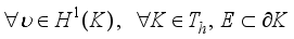 , the following estimates hold
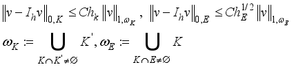

 satisfy the following system.
 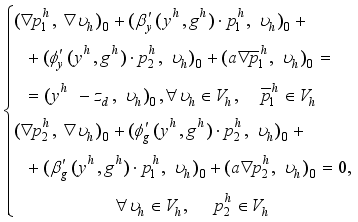 (22)
(22)  is the solution of the system of equations.
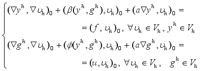
 by
by  .)
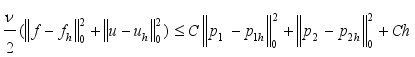
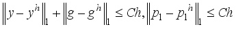
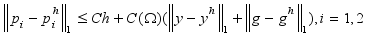
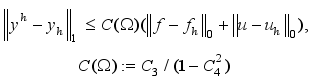
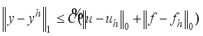
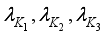
.)  be the solution of (3), (18), respectively. And let us assume that
  . Then the following a priori error estimate holds.
 (23)
(23) 
 .
.  , and using lemma 3, assumption 1 and the above estimate, then we can write
 .
.  , and using lemma 3, assumption 1, then we can write
 (24)
(24)  .
.  , we have
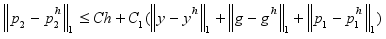
 (25)
(25)  satisfy, we have
 and applying assumption 1, we have
 satisfy, we have
 and applying assumption 1, we have
 (26)
(26) 
 .
.  satisfy, we have
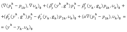
 under exploiting Lipschitz continuity of
  and
and  , we have
 , for
, for  , we have
 (27)
(27) 
 (28)
(28) 
 being
being  .
.  (29)
(29) 
 ,
,  , the solution of (22), we have the following a priori error estimate.
  (30)
(30)  . Because of
  , we can get
  (31)
(31) 
 holds true. We can deduce the second result of lemma in a similar way. So we can complete the proof.
  satisfy the following system.
 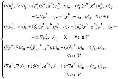 (32)
(32)  and there exists a constant C such that
  (33)
(33)  is an arbitrary point in the neighborhood of
  .
. 
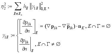
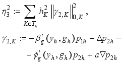
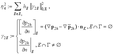
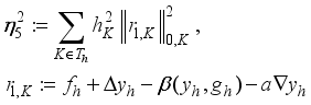
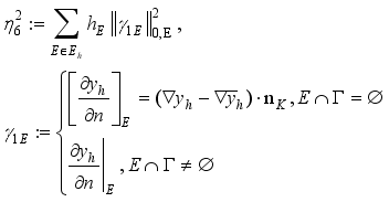
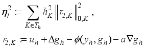
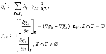
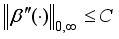
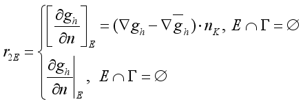
 are the functions defined in (32), C>0 is the constant independent of h.
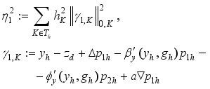
 is the jump of directional derivative on the common boundary E of two elements
  .
. 
 is the jump of directional derivative on the common boundary E of two elements
  .
. 
 is the jump of directional derivative on the common boundary E of two elements
  .
. 
 is the jump of directional derivative on the common boundary E of 2 elements
  .
.  .
.  , let us prove that there is a constant
  independent of v such that
  .
. 
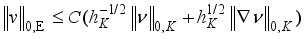
 is the constant in the norm equality
  .
.  , and the inequality
 (34)
(34)  ,
,  . By using the assumption 1 on
  , then we have
 (35)
(35) 
 , we can obtain
 is the equivalence constant between the space
  .
.  , we can deduce
  (36)
(36)  be the solution of (3) and (18), respectively. If the condition
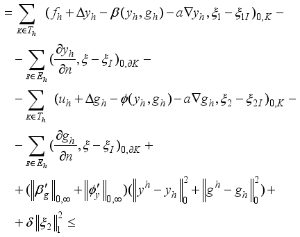
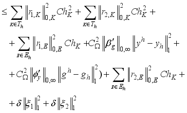
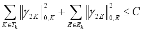
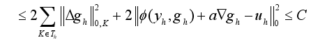
  is valid, then we can obtain the following upper bound estimate for a posteriori error
 (37)
(37)  (38)
(38)  (39)
(39)  , and choosing a trial function as
  , and using assumption 1, then we have
 , and choosing a trial function as
  , using assumption 1 and the monotonity of
  , then we have
 by
by  , and taking into account
  and assumption 1, then it follows that
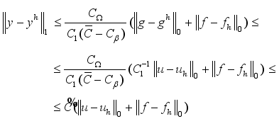
 .
.  , choosing a trial function as
  , taking into account assumption 1, and then we have
 , choosing a trial function as
  , taking into account assumption 1 and above estimations, and then we have
 . Thus there holds
 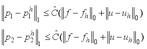 (40)
(40) 
 , which is the common edge of element
  .
. 
 and edge
  , bK, bE have the following characteristics.
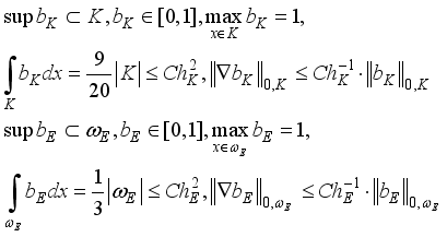
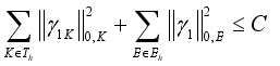
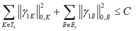
 be the solution of (3), (18). Then we have the following lower bound estimate for a posteriori error by FEM.
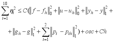
 is independent of
  and two of Cs are not the same.
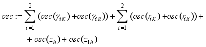
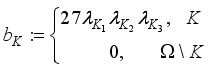
 :
:  .
. 
 .
. 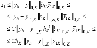
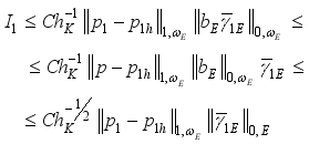
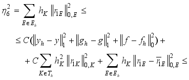
 , we can obtain the following estimates.
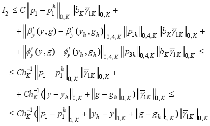
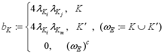
 :
:  .
. 
 .
. 
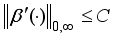
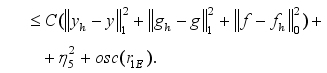
 is taken into account. Likewise, considering the Lipschitz continuity of
  ,
,  , we can deduce the following estimates.
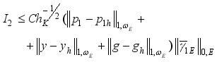
 , we can get the followings.
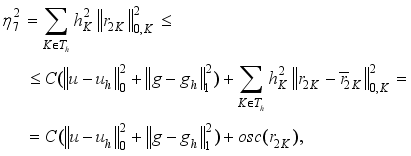
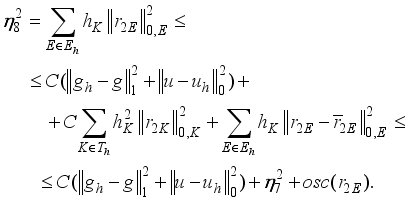
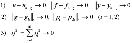
 , we can derive the result of this theorem. This completes the proof.
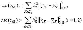
  , oscillation error (Theorem 4),
 are the quantities defined in lemma 7 being
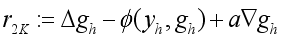
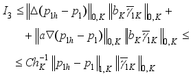
 , it follows that
  is bounded in
  independently of h, i.e.
 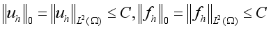 (C is constant independent of h).
  in the variational equation
  (42)
(42)  , and by using assumption 1, lemma 5 and
  , then it follows
 by
by  . Because all finite dimensional norms are equivalent, it follows
 .
.  ,
,  is bounded linear functional in
  , and from Riesz’s representation theorem, there is a unique
  such that
  , and it follows
 (C is independent of h), so we have the following result.
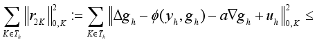
 (43)
(43)  (44)
(44)  (45)
(45)  .
. 
FEM | Finite Element Method |
FVM | Finite Volume Method |
| [1] | Bei Zhang et al, A posteriori error analysis of nonconforming finite element methods for convection-diffusion problems, Journal of Computational and Applied Mathematics, 321, 416-426 (2017). |
| [2] | R. Verfurth, A posteriori error estimates for non-stationary nonlinear convection-diffusion equation, Calcolo, 55, 1-18 (2018). |
| [3] | Chuanjun Chen et al., A posteriori error Estimates of two grid finite volume element method for non-linear elliptic problem, Computers and Mathematics with Applications, 75(2018) 1756-1766. |
| [4] | Xingyang Ye, Chanju Xu, A Posteriori error estimates for the fractional optimal control problems, Journal of Inequalities and Applications, 141(2015), 1-13. |
| [5] | Lin Li et al., A posteriori error Estimates of spectral method for non-linear parabolic optimal control problem, Journal of inequalities and applications, 138(2018) 1-23. |
| [6] | E. Casas et al., Error Estimates for the numerical approximation of Dirichlet boundary control for semilinear elliptic equations, SIAM J. Control Optim., 45(2006) 1586-1611. |
| [7] | D. Y. Shi, H. J. Yang, Superconvergence analysis of finite element method for time-fractional thermistor problem, Appl. Math. Comput., 323 (2018) 31–42. |
| [8] | D. Y. Shi, H. J. Yang, Superconvergence analysis of nonconforming FEM fornonlinear time-dependent thermistor problem, Appl. Math. and Compu., 347 (2019) 210–224. |
| [9] | Y. Chen, L. Chen, X. Zhang, Two-grid method for nonlinear parabolic equations by expande mixed finite element methods, Numer. Methods Part. Diff. Equ., 29(2013) 1238-1256. |
| [10] | Meyer C., Error estimates for the finite element approximation of an elliptic control problem with pointwise state and control constraints, Control and Cybern., 37(1), 51-83 (2008). |
| [11] | Wollner W., A posteriori error estimates for a finite element distretization of Interior point methods for an elliptic optimization problem with state constraints, Numer. Math. Vol. 120, No. 4, 133-159 (2012). |
| [12] | Rosch, D. Wachsmuth, A posteriori error estimates for optimal control problems with state and control constraints, Numerische Mathematik, Vol. 120, No. 4, 733-762 (2012). |
| [13] | Benedix, B. Vexler, A posteriori error estimation and adaptivity for elliptic optimal control problems with state constraints, Comput. Optim. Appl., 44(1), 3-25 (2009). |
| [14] | Dib S., Girault V., Hecht F. and Sayah T., A posteriori error estimates for Darcy’s problem coupled with the heat equation, ESAIM Mathematical Modelling and Numerical Analysis, |
| [15] | Allenes, E. Otarola, R. Rankin. A posteriori error estimation for a PDE constrained optimization problem involving the generalized Oceen equations, SIAM J. Sci. Comput., Vol. 40, No. 4, A2200-A2233, 2018. |
| [16] | Natalia Kopteva. Error analysis of the L1 method on graded and uniform meshes for a fractional-derivative problem in two and three dimensions. Math. Comp., 88(319): 2135–2155, 2019. |
| [17] | Xiangcheng Zheng and Hong Wang. Optimal-order error estimates finit element approximations to variable-order time-fractional diffusion equations without regularity assumptions of the true solutions. IMA J. Numer. Anal., 41(2): 1522–1545, 2021. |
| [18] | Natalia Kopteva. Pointwise-in-time a posteriori error control for time-fractional parabolic equations. Appl. Math. Lett., 123: Paper No. 107515, 8, 2022. |
APA Style
Kim, C., Ri, J., Kim, S. J. (2025). A Posteriori Error Estimates by FEM for Source Control Problems Governed by a System of Semi-Linear Convection-Diffusion Equations. International Journal of Industrial and Manufacturing Systems Engineering, 10(2), 20-35. https://doi.org/10.11648/j.ijimse.20251002.11
ACS Style
Kim, C.; Ri, J.; Kim, S. J. A Posteriori Error Estimates by FEM for Source Control Problems Governed by a System of Semi-Linear Convection-Diffusion Equations. Int. J. Ind. Manuf. Syst. Eng. 2025, 10(2), 20-35. doi: 10.11648/j.ijimse.20251002.11
AMA Style
Kim C, Ri J, Kim SJ. A Posteriori Error Estimates by FEM for Source Control Problems Governed by a System of Semi-Linear Convection-Diffusion Equations. Int J Ind Manuf Syst Eng. 2025;10(2):20-35. doi: 10.11648/j.ijimse.20251002.11
@article{10.11648/j.ijimse.20251002.11,
  author = {ChangIl Kim and JaYong Ri and Song Jun Kim},
  title = {A Posteriori Error Estimates by FEM for Source Control Problems Governed by a System of Semi-Linear Convection-Diffusion Equations
},
  journal = {International Journal of Industrial and Manufacturing Systems Engineering},
  volume = {10},
  number = {2},
  pages = {20-35},
  doi = {10.11648/j.ijimse.20251002.11},
  url = {https://doi.org/10.11648/j.ijimse.20251002.11},
  eprint = {https://article.sciencepublishinggroup.com/pdf/10.11648.j.ijimse.20251002.11},
  abstract = {In this paper, we consider the optimal source control problem of a system of 2-dimensional semi-linear steady convection-diffusion equations. The problem is modelized from temperature and consistency distribution in the gasification processes, so it is described by 2 non-linear elliptic partial differential equations with Dirichlet boundary condition. The problem is a optimal source control problem that controls the source term necessary to approximate the temperature to a proper target function. First, we derived the optimal condition. Based on setting the approximation problem of a given control problem in a first order polynomial finite element function space and deriving the optimality condition of the approximation problem, we evaluated a priori error between the optimal control, the optimal state, the conjugate state and its finite element approximation functions by using optimal condition of original and approximate problem. And we also evaluated the upper estimate of a posteriori error by finite element method (FEM). We proved the convergence to 0 of a posteriori error indicator (term of the right side of inequality) when division diameter converges to 0. For this, we acquired the lower bound estimation of a posteriori error and proved that a priori error and total variance error converges to 0 when division diameter converges to 0, so that we proved the convergence problem of a posteriori error indicator.
},
 year = {2025}
}
TY  - JOUR
T1  - A Posteriori Error Estimates by FEM for Source Control Problems Governed by a System of Semi-Linear Convection-Diffusion Equations

AU  - ChangIl Kim
AU  - JaYong Ri
AU  - Song Jun Kim
Y1  - 2025/09/23
PY  - 2025
N1  - https://doi.org/10.11648/j.ijimse.20251002.11
DO  - 10.11648/j.ijimse.20251002.11
T2  - International Journal of Industrial and Manufacturing Systems Engineering
JF  - International Journal of Industrial and Manufacturing Systems Engineering
JO  - International Journal of Industrial and Manufacturing Systems Engineering
SP  - 20
EP  - 35
PB  - Science Publishing Group
SN  - 2575-3142
UR  - https://doi.org/10.11648/j.ijimse.20251002.11
AB  - In this paper, we consider the optimal source control problem of a system of 2-dimensional semi-linear steady convection-diffusion equations. The problem is modelized from temperature and consistency distribution in the gasification processes, so it is described by 2 non-linear elliptic partial differential equations with Dirichlet boundary condition. The problem is a optimal source control problem that controls the source term necessary to approximate the temperature to a proper target function. First, we derived the optimal condition. Based on setting the approximation problem of a given control problem in a first order polynomial finite element function space and deriving the optimality condition of the approximation problem, we evaluated a priori error between the optimal control, the optimal state, the conjugate state and its finite element approximation functions by using optimal condition of original and approximate problem. And we also evaluated the upper estimate of a posteriori error by finite element method (FEM). We proved the convergence to 0 of a posteriori error indicator (term of the right side of inequality) when division diameter converges to 0. For this, we acquired the lower bound estimation of a posteriori error and proved that a priori error and total variance error converges to 0 when division diameter converges to 0, so that we proved the convergence problem of a posteriori error indicator.

VL  - 10
IS  - 2
ER  -
Department of Mathematics, University of Sciences, Pyongyang, DPR Korea
Department of Mathematics, University of Sciences, Pyongyang, DPR Korea
Department of Mathematics, Pyongsong University of Education, Pyongsong, DPR Korea


 Under this assumption, y, g, the solutions of (
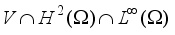
 of
of  , the solution of (
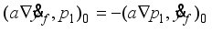 , then we have
  , we have the equality
  , then we have
  is the solution of (
 be the solutions of (
 , where
  is the solution of (
 , the solutions of (
 .
.  be the solution of (
 be the solution of (
 .
.  , by summing up (
 be the solution of (